Feature View
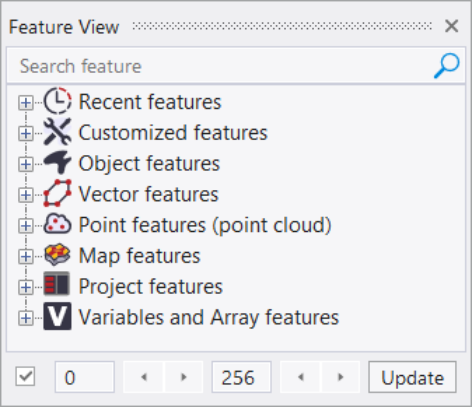
Once you have created image objects you can visualize feature values based on Tools > Feature View. Additionally, you can implement your own features based on customized features. eCognitions features are grouped in these main sections:
- Recent features
- Customized features
- Object features
- Vector features
- Point features (point cloud)
- Map features
- Project features
- Variables and Array features
For more details see Reference Book > Features - Overview.
Segmentation Preview
This tool helps you to choose and calibrate a segmentation algorithm of your choice, and to test different parameters effectively on a subset that displays the potential objects. Once appropriate values are found, the algorithm is inserted in the process tree and can be applied to the whole scene.
This saves users time since the parameter calibration is not performed for the entire scene. As opposed to the workaround of creating a scene subset for testing the segmentation parameters, this tool allows more flexibility as the segmentation preview window can be easily moved to any location in the scene.
Please take a look at the video: Segmentation Preview
To open the Segmentation Preview select:
-
Tools > Segmentation Preview or
-
in the Process Tree > Add new process. In the Edit Process window, choose a segmentation algorithm and press the Segmentation Preview button in the lower left corner of the window.
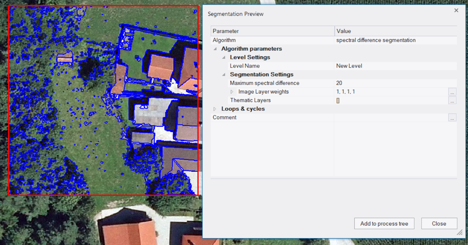
Now a red rectangle is displayed in the active view that shows image objects based on the chosen parameters. In the Segmentation Preview window, choose the segmentation type to be displayed using the drop-down Parameter > Algorithm (default multiresolution segmentation). Depending on the selected segmentation algorithm the available parameters change (for parameter details, please see respective algorithm in the Reference Book).
Following segmentation algorithms are available in the segmentation preview tool:
-
cheessboard segmentation
-
quadtree based segmentation
-
contrast split segmentation
-
vector-based segmentation
-
stddev split segmentation
-
multiresolution segmentation (default)
-
spectral difference segmentation
-
multi-threshold segmentation
-
superpixel segmentation
-
contrast filter segmentation
-
watershed segmentation
If you change one of the parameter values, the preview window is updated on the fly and the image objects reflect the new settings immediately.
You can move the red rectangle or change its size with your mouse in Normal Cursor mode.
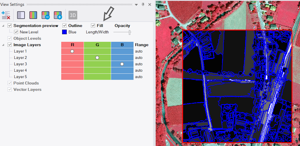
Additionally, with the Segmentation Preview window open, you can change the outline color or fill color and opacity in the View Settings dialog. If you select a Feature Value for fill type, the image objects reflect the feature values in grey tones in the preview rectangle.
Once the segmentation algorithm is calibrated, use the Add to process tree button to insert a new process or to insert the modified process into the process tree - If you opened the Segmentation Preview window using:
-
Tools > Segmentation Preview - this button will insert a new segmentation process with the selected parameters into the process tree.
-
Process Tree > Add new process > Edit Process > Segmentation Preview - this button will update and overwrite the parameters of an existing algorithm in the process tree.
that the objects of the segmentation preview can differ slightly from objects based on a real segmentation because of border effects.
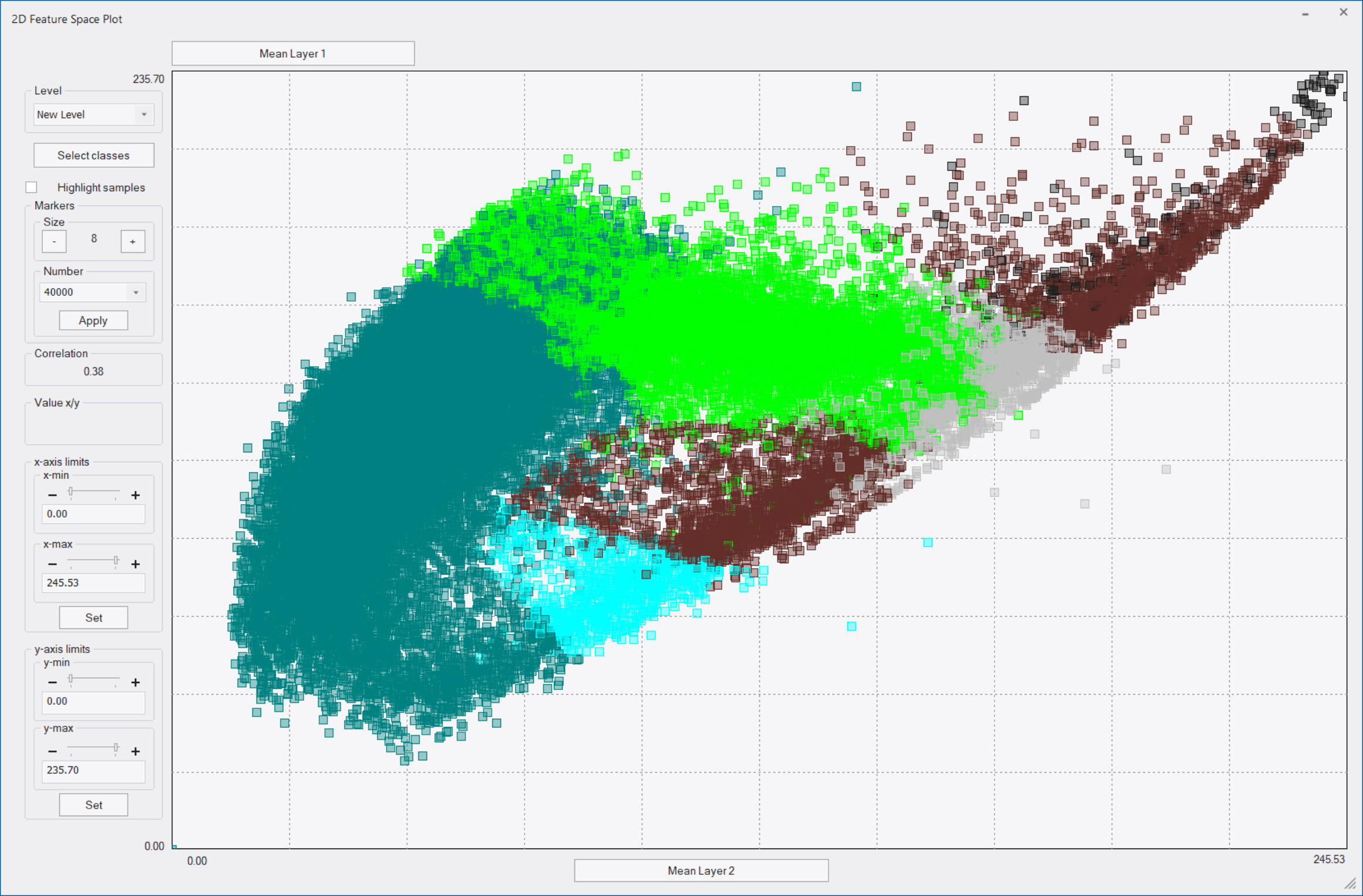
2D Feature Space Plot
This tool displays markers in a scatter plot to represent values for two selectable features. Each marker represents an image object or sample. The 2D Feature Space Plot is used to observe relationships between features, obtain information on the distribution and patterns of image objects, and outlier points. It provides information on classified image objects, highlights samples and shows the correlation of two features.

Feature Y Axis - Button to select the feature for the y-axis (default: Standard deviation Layer 1).
Level - Select the image object level of interest.
Select classes - Select the classes to display.
 Highlight samples - Option to highlight existing samples.
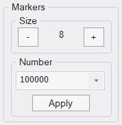
Markers - Change the size and number of markers in the scatter plot to improve visualization. Reduce the size and amount of markers so that fewer overlaps occur for the selected level.
Size - Display size of square markers (range 1-19, default value 8).
Number - Number of markers visualized (default 10000). If the number of image objects is larger than 10000 only a random selection of image objects is visualized by default. Select all in the drop-down to render all existing image objects or enter a value directly in the field and select the Apply button.
Correlation - Correlation coefficient (Pearson) to measure the linear correlation for the selected features, calculated for the selection of visualized image objects (defined in number of markers) and for selected classes. It describes the strength and direction of the relationship between the two selected features.
Value x/y - Value of x-axis and y-axis feature in the scatter plot for the current location of the mouse pointer.
x-axis limits - Sets the x-axis limits.
x-min - Minimum limit for x-axis.
x-max - Maximum limit for x-axis.
y-axis limits - Set the x-axis limits.
y-min - Minimum limit for y-axis.
y-max - Maximum limit for y-axis.
Feature X Axis - Button to select the feature for the x-axis (default: Mean Layer 1).
Accuracy Assessment Tools
Accuracy assessment methods can produce statistical outputs to check the quality of a classification result regardless of the method used to classify the image objects.

- Choose Tools > Accuracy Assessment on the menu bar to open the Accuracy Assessment dialog box.
- In the Confusion Matrix drop-down list, select one of the following methods for accuracy assessment:
samples - select if you want to calculate and visualize the confusion matrix based on sample objects within a single project.
file (flattened) - select if you want to calculate and visualize the confusion matrix across multiple projects within the workspace based on the exported flattened confusion matrix results.
object variable - select if you want to calculate and visualize the confusion matrix based on objects defined as samples via an object variable within a single project.
- A project can contain different classifications on different image object levels. Specify the Image object level of interest by using the level drop-down menu.
- A project can contain ground truth information stored in Image object variables. For the selection of Confusion Matrix based on object variable select the corresponding variable name in this drop-down menu. This option is only activated for selection of Confusion Matrix based on object variable.
- Classes - To select classes for assessment, click the Select classes button and make a new selection in the Select Classes for Statistic dialog box. By default all available classes are selected. You can deselect classes through a double-click in the right frame.
- Load file (flattened)- This option is only activated for the selection of Confusion Matrix based on file (flattened) and lets you import and visualize an existing flattened file. This file can be created using the export algorithm Export Confusion Matrix .
- To view the accuracy assessment results, click Show statistics. To export the statistical output, click Save statistics. Enter a file name in the File name field and save the table in *.csv, *.txt or *.tcsv file format. The statistics file will be saved in the workspace root folder by default.
Confusion Matrix
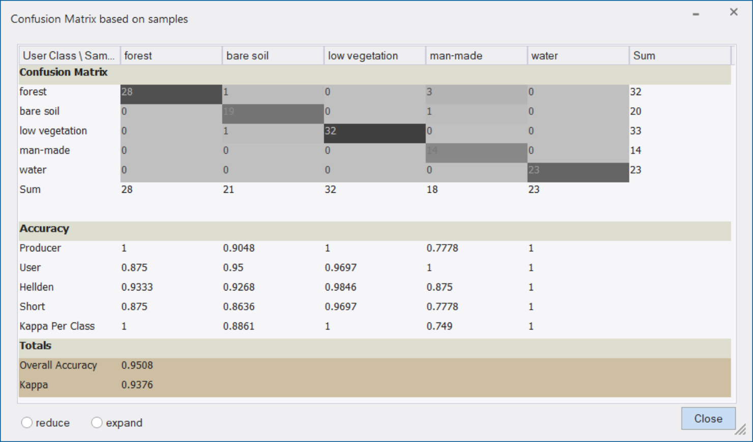
The Confusion Matrix dialog box displays different statistic types used for accuracy assessment.
Test areas are used as a reference to check classification quality by comparing the classification with reference values (called ground truth in geographic and satellite imaging) based on pixels.
This statistic type considers samples (not pixels) derived from sample inputs. The match between the sample objects and the classification is expressed in terms of parts of class samples.
The Confusion Matrix dialog box displays the following statistics used for accuracy assessment:
User Class / Sample
The vertical column shows the user classes. The rows in horizontal direction reflect the sample/reference data.
Sum
The Sum row shows the number of objects/pixels that should have been identified as a given class, according to the sample/reference data.
Producer
The producer's accuracy is a false negative, where objects/pixels of a known class are classified as something other than the reference class.
User
The user's accuracy calculates false positives, where objects/pixels are incorrectly classified as a known class.
Hellden
The Hellden index is a mean accuracy index and denotes the probability of a randomly chosen point of a user class and its correspondence of the same class in the same position in the sample/reference data.
Short
The Short’s mean accuracy calculates the ratio of the estimated and sample/ ground truth classes intersection to their union.
Kappa per class
The Cohen's Kappa coefficient (see below) identifies the agreement that is expected when classes are totally independent while Kappa per class calculates the same agreement at per-classes level.
Overall accuracy
The overall accuracy calculates the proportion of pixels out of the reference sites/ground truth sites that were mapped correctly. The overall accuracy is usually expressed in percent, with 100% accuracy being a perfect classification - all reference objects were classified correctly. Range [0,1].
Cohen's Kappa
The Kappa coefficient measures the agreement between two sets - a classification result and ground truth objects/samples, while correcting for agreement that occurs by chance. This statistic is useful for measuring the predictive accuracy in a classification matrix. The Kappa coefficient can range from [-1 , 1], where a value for K = 0 is obtained when the agreement equals chance agreement and the upper limit of Kappa (+ 1.00) occurs only when there is perfect agreement between the two sets.
Related to:
-
Video - Accuracy Assessment
-
algorithm Export Confusion Matrix
-
algorithm Compute Accuracy Values
Projection and Reprojection
Assign Projection
If the coordinate system of a dataset is unknown or incorrect you can use this tool to assign a projection Tools > Projection > Assign Projection, under the precondition that you know the projection information.
Existing information on the coordinate system stored in the dataset will be overwritten. This tool does not reproject data and or perform any calculations. To reproject data open the dialog Tools > Projection > Reproject Data.
Supported data formats are tif for image data, shapefile for vector data and point clouds in LAS and LAZ formats.
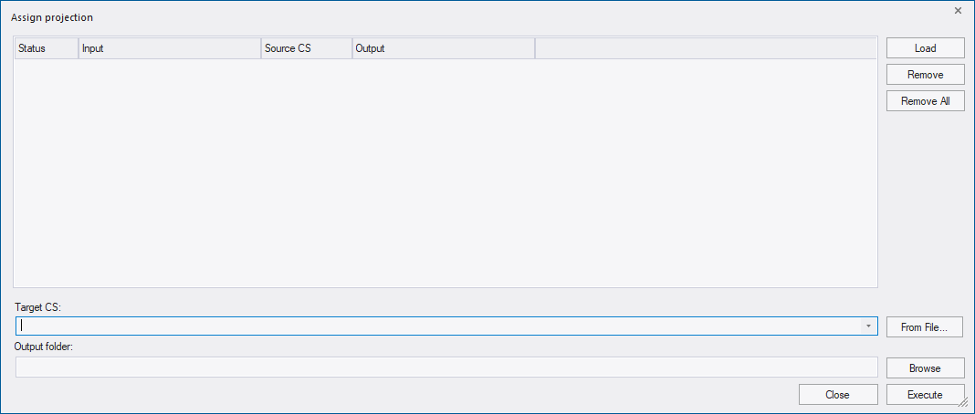
First step is to add the data to the dialog by clicking the Load button.
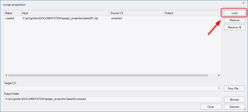
Following information is displayed for each file:
- Status - returns the current status of the input file:
- Loaded - data layer has been successfully added
- Processing - defined projection is being assigned
- Canceled- projection assignment has been interrupted by user
- Finished - defined projection has been successfully assigned to the data
- Input - path to file location
- Source CS - coordinate system of the input file
- Output - ouput path for the processed file
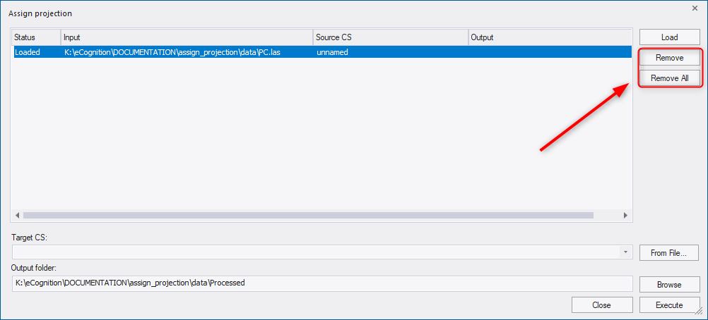
To remove a data file from the list, select the file and press the Remove button. To remove all files from the list, press the Remove All button. These two functionalities do not delete the file, the file will be just unloaded from the list of this Assign Projection dialog.
The target coordinate system (Target CS) can be selected or searched from the drop-down list . To search for a coordinate system, start typing a name or an EPSG code of a coordinate system in the field. Alternatively, a target coordinate system can be loaded via file using the From File button to the right of the drop-down.
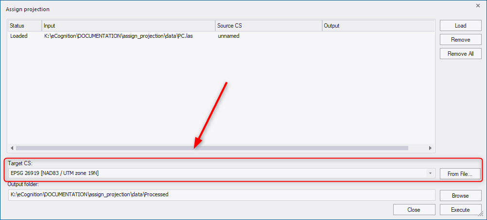
The target coordinate system must be a projected coordinate system. Supported input formats are tif, shp, LAS/LAZ (see also Reprojection tool in following chapter).
In the Output folder field, the path for files with assigned projection is displayed: by default they are located in a subfolder of the data folder called Processed. (If the data is located in different folders, the default path is the folder of the first loaded dataset). However, you can define the ouput folder using the Browse button or type directly into the Output folder field.
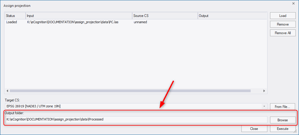
To assign the new projection to the loaded input files, press the Execute button. Then a progress bar appears on the screen indicating the status of processing. When the projection assignment is done an output path appears next to each file in the dialog.
Reproject
For image analysis in eCognition Developer, the data used must belong to the same projected coordinate system. Geographic coordinate systems have different pixel size in X and Y axes resulting in non-square pixels which should be avoided.
This reprojection tool can be used for reprojecting data from a geographic coordinate system to a projected coordinate system or from one projected coordinate system to another if the data are defined on different systems or if you need the results in a coordinate system different from the one of the input data.
To reproject data select Tools > Projection > Reproject Data.
Supported data formats are tif for image data and shapefile format for vector data.
Use the Load button to add the data to the Reproject data dialog.
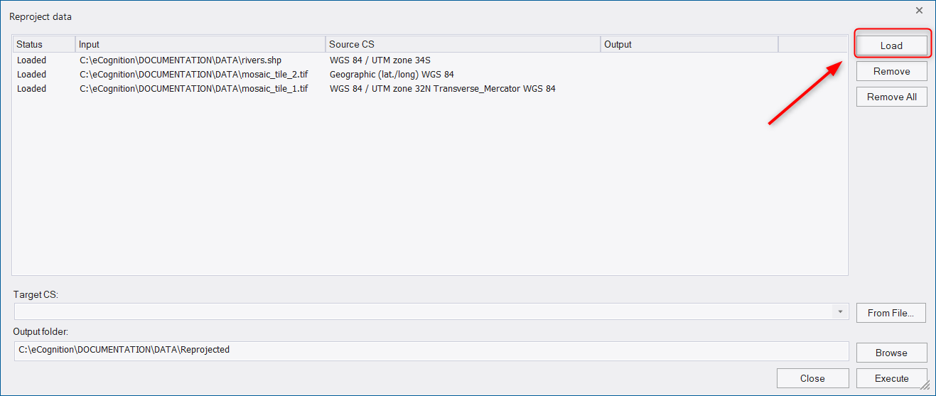
In the dialog you get the following information for each file:
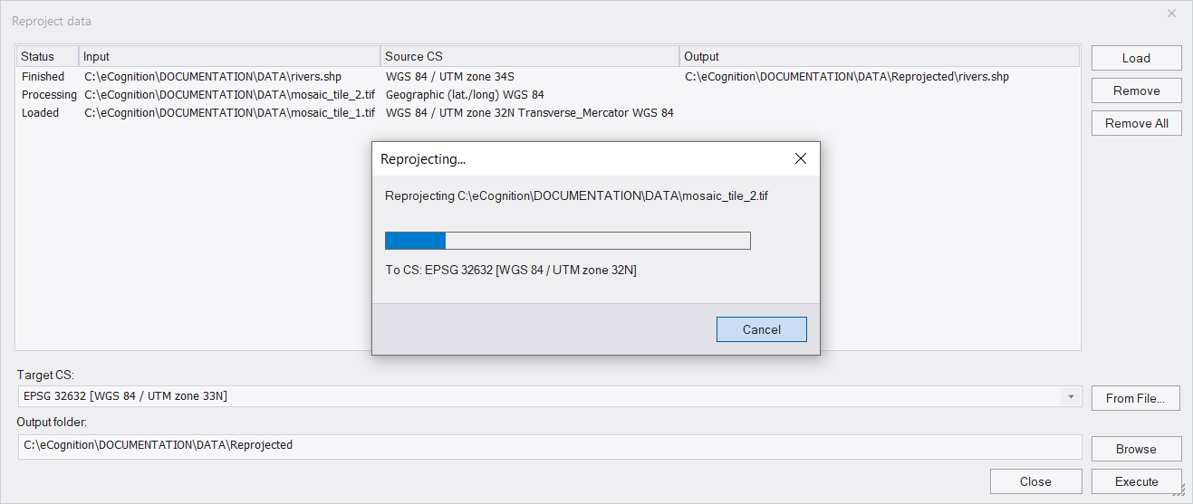
- Status - returns the current status of the input file:
- Loaded - data layer has been successfully added
- Processing - target coordinate system is being reprojected
- Canceled - reprojection has been interrupted by user
- Finished - reprojection has been successfully executed
- Input - the path to the file location
- Source CS - coordinate system of the input file
- Output - path to the reprojected file
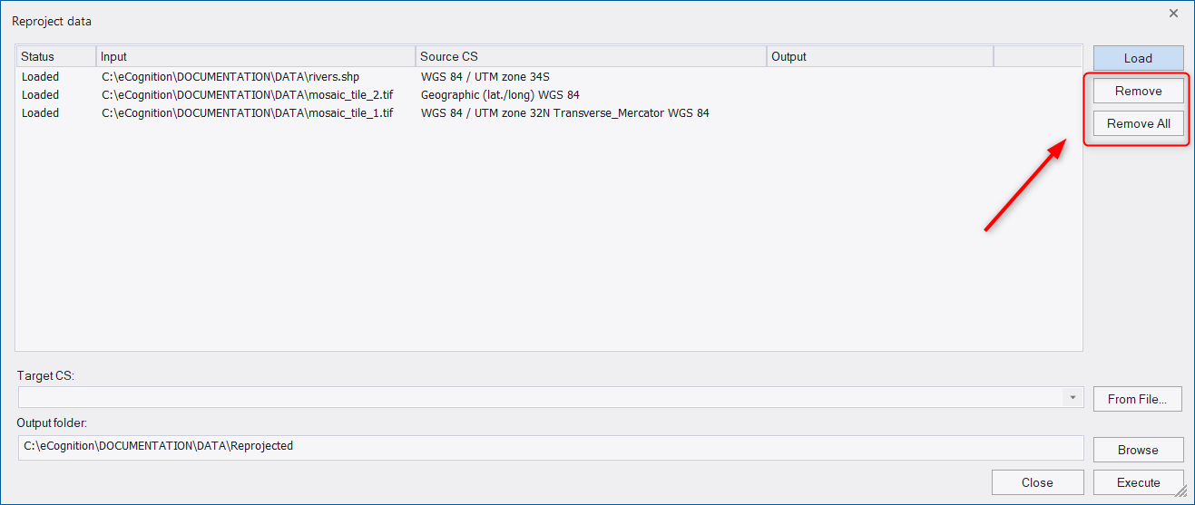
To remove a data file from the list, select the file and press the Remove button. To remove all files from the list, press the Remove All button. These two functionalities do not delete the file, the file will be just unloaded from the list of the Reproject dialog.
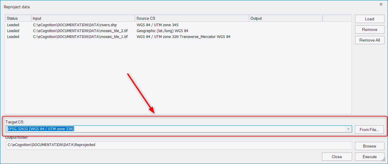
The target coordinate system (Target CS) can be selected or searched from the drop-down list. To search for a coordinate system, start typing a name or an EPSG code of a coordinate system in the field. Alternatively, a target coordinate system can be loaded via file using the From File button to the right of the drop-down.
The target coordinate system must be a projected coordinate system. Supported data formats are TIF for image data and shapefile for the vector data.
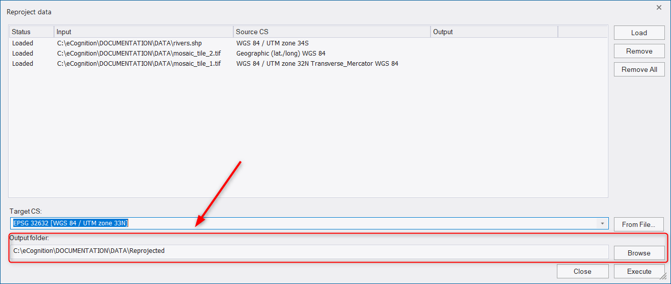
In the Output folder field, the path for reprojected files is displayed: by default they are located in a subfolder of the data folder called Reprojected. (If the data is located in different folders, the default path is the folder of the first loaded dataset). However, you can define the ouput folder using the Browse button or type directly into the Output folder field.
To reproject the loaded input files press the Execute button.
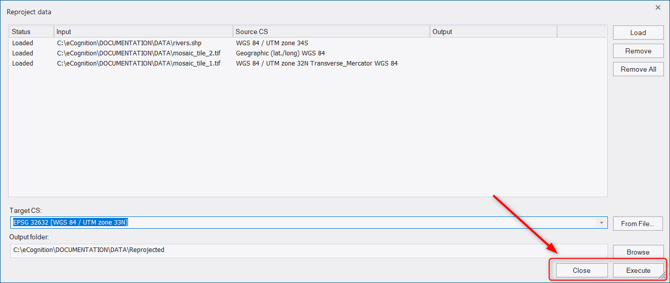
Then a progress bar appears indicating the status of processing. Once the reprojection is applied an output path appears next to each file in the dialog window.
If you add image layers or thematic layers to a project, that are assigned to a geographic coordinate system, a warning message is prompted that it is recommend to reproject the data. Select one of the following options:
- Continue: add data without reprojection
- Assign projection: assign a projection to the data without reprojecting it
- Re-project: reproject data using the reprojection tool (adds data automatically to the workspace)
- Cancel: do not add the data and exit the dialog
